First Steps With Text Analysis
This is the beginning of experimentation with a new topic: text analysis! I have always heard about text analysis or natural language processing (NLP) for quite some time, but I never learned anything about it. So, it is about time I got started…
First resource
Since I mostly code in R, it was a natural choice to use it as a platform for my learning. The book “Text Mining with R: A Tidy Approach” seemed like a good choice for a starting point.
At the time of writing this post, I have completed reading and coding along 4 chapters that introduced the following topics:
-
The tidy text format which follows the famous “tidy” table format by having one row per word (or token).
-
Tokenization of text documents, i.e., splitting them into tokens. Tokens are either single words (unigrams) or pieces with more than one words (n-grams).
-
Sentiment analysis by giving tokens labels or scores to reflect the positive/negative sentiment, which are then analyzed.
-
Analyzing frequency and tf-idf as a measure of token importance in a document.
-
Network/graph visualization to explore relationships between words.
Some output
Let me share some of the nice analysis results that I made. They use almost the same code from the book, with a few visual tweaks here and there.
Sentiment analysis

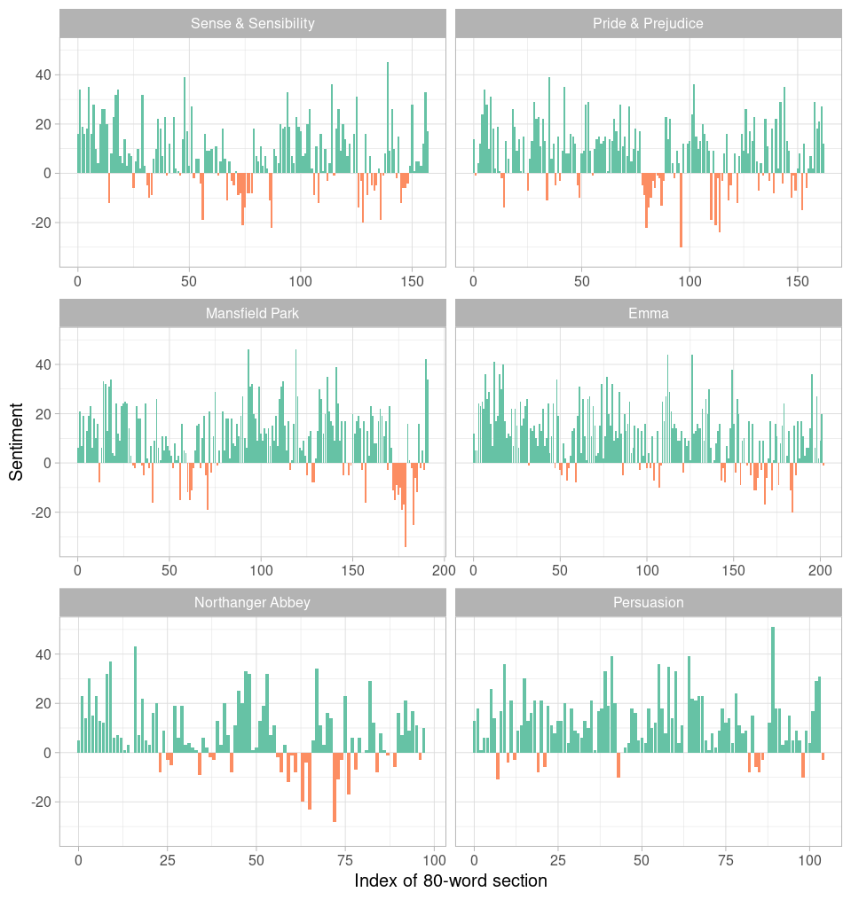
The first one is the result of sentiment analysis of books by dividing the book into 80-word sections and calculating the sentiment score of each section. For example, the book “Mansfield Park” has mostly words of positive sentiment. But it reverses near the end into negative sentiment and finally back to positive.
Note that in this basic example, negation is not accounted for. In other words, something like “not good” still counts as a positive sentiment because “good” does.
Bigram network

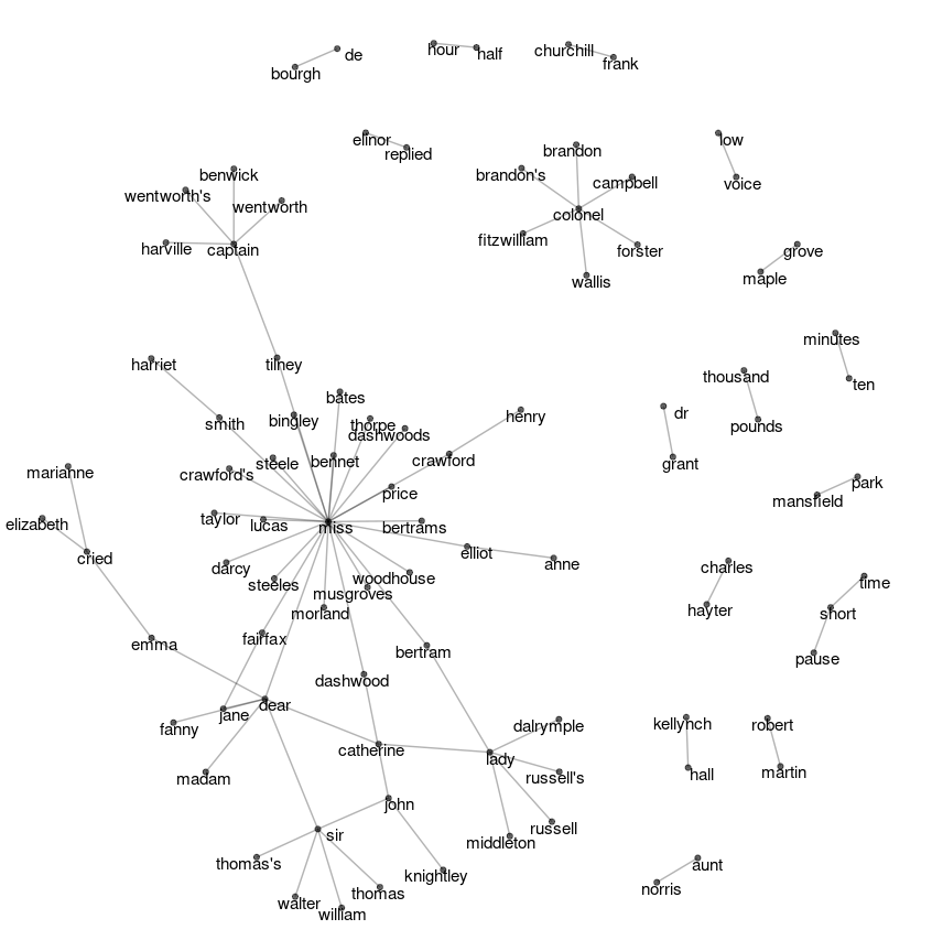
Just like text analysis/NLP, network visualization is something I never tried before. So, it was nice to try it out here. This here is a simple one that shows common co-occurrences between pairs of words (bigrams).
Unsurprisingly, most bigrams are either first and last names or a single name associated with a title like “miss”, “dr”, or “captain”.
Zipf’s law

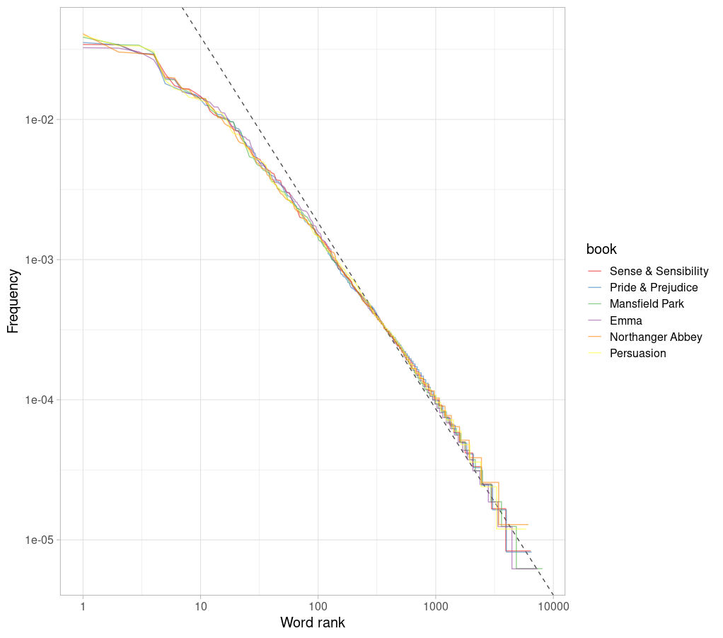
This one is interesting. Zipf’s law states that in a book or a similar collection of words, the second most frequent word is half as frequent as the most common word, the third most frequent is a third as frequent, and so on. To put it succinctly: $$frequency \propto \frac{1}{rank}$$
It does show in the analyzed set of books, although there is some divergence in the most common words, i.e., they are used less frequently than what would be expected from Zipf’s law.
P.S. It reminded me of a Vsauce video…
Reflection and goals
I was able to pick up the basics of text analysis using these few chapters. I find it just as interesting as any other data analytic topic. The obvious next step for me will be to continue reading the book and practice with the case studies that are provided there.
Finally, there is one single application that interests me at the moment, and that is searching. More specifically, I am looking forward to make an implementation that:
-
Takes some user input and search for it in a pre-specified text dataset.
-
Works like web search engines which give the results that match all the input keywords (if any), then the results that match fewer keywords, and so on.
-
Allows fuzzy matching, i.e., the input can be misspelled, and the matched results are sorted by similarity.
I am not sure that the ideas behind an algorithm like this will be covered in the book. Also, I doubt that I will need machine learning for this, because I am not trying to make predictions – I only need it to look for the closest match in a finite set of choices. However, machine learning might be needed in a more advanced application in which the search keywords are extracted from full sentences/paragraphs of user input.
